Instructions to participate
Table of Contents
To participate, please find below the description of the experiments. The intercomparison is divided into six suites A-F which themselves consist of several runs, e.g. A1-A6.
There are also technical details, such as where to find input-files, how to submit test-runs, how to include your model setup in the official repository, etc.
| Suite | Geometry | Temporal | Varying parameter | Remarks |
|---|---|---|---|---|
| A | sqrt | steady | input volume | maybe fit to A3 and A5 |
| B | sqrt | steady | moulin density | |
| C | sqrt | diurnal | diurnal amplitude of moulins | use B5 as initial condition (IC) |
| D | sqrt | seasonal | -4 to +4C temperature | use A1 as IC |
| E | valley | steady | geometry change | |
| F | valley | seasonal | -6 to +6C temperature | IC: steady state using only winter discharge |
Model parameters and tuning
The aim of this inter-comparison is to obtain results –from models employing a variety of different drainage physics– which are qualitatively comparable. This we hope to achieve by specifying a set of parameters and a tuning strategy, when the parameters are not sufficient or misleading.
Note that we report all quantities in SI-units kg, m, s.
Parameters
We distinguish between "physical constants" (first table) and "parameters" (second table). The former should not be used for tuning whereas the latter can be used if needs be. We suggest that most poorly constraint parameters should be used for tuning, i.e. probably the ones directly related to water flow.
The given parameters are based on the ones used by the GlaDS-model
(Werder et al. 2013), therefore, please report the different
parameters your model uses and we can include them here. Script files
containing the parameters are located in the parameters/ folder in
the bitbucket repository.
| Name | Value |
|---|---|
| Density water | 1000 kg m-3 |
| Density glacier (ice+firn) | 910 kg m-3 |
| Accel. gravity | 9.8 m s-2 |
| Latent heat of fusion | 334 kJ kg-1 |
| Specific heat capacity water | 4220 j kg-1 K-1 |
| Clausius-Clapeyron constant | 7.5e-08 K Pa-1 |
| Seconds per year | 365 *24 *60 *60 s |
| Name | Value | Reference/remarks |
|---|---|---|
| Ice flow | ||
| Glen's n | 3 | |
| Ice flow constant A | 3.375e-24 Pa-3 s-1 | see note after table |
| Ice sliding speed | 1e-6 m s-1 | Werder et al. 2013 |
| Bedrock bump wave-length | 2 m | Werder et al. 2013 |
| Bedrock bumps height | 0.1 m | Werder et al. 2013 |
| Water flow | ||
| Turbulent flow exponent \(\alpha\) | 1.25 | Werder et al. 2013 |
| Turbulent flow exponent \(\beta\) | 1.5 | Werder et al. 2013 |
| Conductivity sheet \(k_s\) | 0.005 m7/4 kg-1/2 | Werder et al. 2013 |
| Sheet-width contributing to R-channel melt | 2 m | Werder et al. 2013 |
| Englacial void fraction | 0 (sqrt) 1e-3 (valley) | Werder et al. 2013 |
| Conductivity R-channel \(k_c\) | 0.1 m3/2 kg-1/2 | Werder et al. 2013 |
| Darcy-Weisbach equivalent of \(k_c\) | 0.195 | for semi-circular R-channel |
Note that the ice flow constant \(A\) is for the usual channel closure relation of the form \(\frac{\partial S}{\partial t}=\frac{2A}{n^n} SN^n\) with channel cross-sectional area \(S\), effective pressure \(N\) and Glen's \(n\). This is how \(A\) is usually defined, e.g. in Cuffey & Paterson 2010. In the GlaDS paper a closure relation of the form \(\frac{\partial S}{\partial t}=A' SN^n\) is used, and the value of the constant is then \(A'=\) 2.5e-25 Pa-3 s-1.
Tuning
To obtain comparable results for different models we suggest to use test case A3 and A5 as a "common ground", which is achieved by tuning models to the output of GlaDS (see figures below and provided as ascii files for A3 and A5). The focus should lie on tuning to the effective pressure \(N\), but sheet \(q\) and channel discharge \(Q\) can also be used (please indicate in the questionnaires).

Figure 1: Model run A3 (left) and A5 (right) of GlaDS: effective pressure (mean enveloped by min/max), sheet discharge (mean enveloped by min/max), and channel discharge (max).
The parameters thus obtained are then used for the subsequent experiments. A3 is chosen as a case where GlaDS (for the used parameters) produces a distributed system only, whereas A5 features channelisation up to around mid-domain.
Models which do not include both inefficient and efficient drainage may need to use a different set of parameters to tune to A3 and A5. Or may choose to only apply the model to part of the test cases.
If you feel that your model should not or cannot be tuned to A3 and/or A5, then run the model with the most appropriate set of parameters. However, in such a case it is encouraged to submit two sets of results: one tuned as best as possible and one using the most natural set of parameters.
Geometries & boundary conditions
The test geometries have been defined in a simple way to allow the participation of both flowline/flowband and 2D map plane models. The reference implementation can be found in the file topo.jl, which also contains plotting routines for visualisations. In the same folder implementations in other programming languages can also be found (please contribute if you write a new one).
"sqrt": ice-sheet margin-like geometry
This geometry is used for the suites A-D and mirrors a synthetic land-terminating ice sheet margin as was used in Werder et al. 2013, but with a few modifications. The domain is 100km long in the \(x\) direction and 20km wide in the \(y\) direction with the terminus along \(x=0\). The bedrock is a flat surface at 0m elevation and the surface is defined by a square root function1:
surface(x,y) = 6*( sqrt(x+5e3) - sqrt(5e3) ) + 1
bed(x,y) = 0
This means that the maximal ice thickness is 1521m, and minimal 1m.
One dimensional models (1D) should use the following functions:
# 1D models
surface(x) = surface(x,0)
bed(x) = 0
width(x) = 20e3
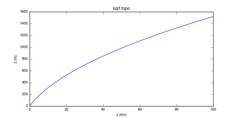
Figure 2: Side view of sqrt topography
"sqrt": boundary conditions
The boundary conditions should be set such that there is no influx along the interior boundaries (i.e. \(y=0\), $y=20$km, $x=100$km). Water pressure should not need specifying along the interior edges, if your model requires this, please mention it in the questionnaires. At the margin edge (\(x=0\)), set pressure to 0Pa. No boundary condition on the flux should be needed, allowing for free outflow.
"valley": Bench Glacier-like geometry
The two suites E & F are performed on a 2D valley geometry to
investigate the impact of the smaller glacier-size and of the bedrock
shape on the behavior of the models. The geometry is based on the
shape of Bench Glacier (Alaska, approximately 6km by 1km). The
bed-geometry has one parameter para which determines whether the bed
has an overdeepening or not, with para=0.05 mimicking Bench Glacier
with no overdeepening.
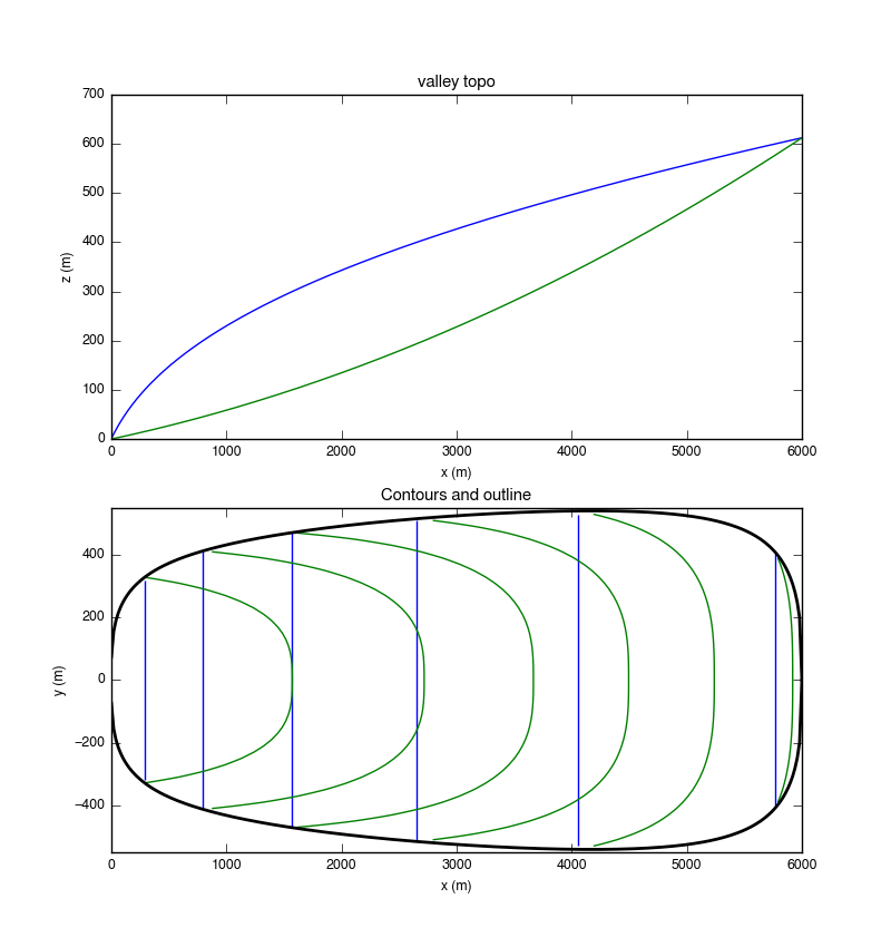
Figure 3: valley topography with para=0.05: side view (top) and map view (bottom, contours 100m).
The defining functions are
surface(x,y) = 100(x+200)^(1/4) + 1/60*x - 2e10^(1/4) + 1
bed(x,y, para) = f(x,para) + g(y) * h(x,para)
with the helper functions f(x,para), g(x,para), and h(x,para).
f determines the flow-line geometry and it is constructed such that
f(6e3, para)==surface(6e3,0), i.e. the ice thickness is always 0 at
the upper end of the glacier (=6e3m). g determines the
cross-sectional geometry which is modified by h. The function h
is chosen such that the glacier outline is independent of para.
They are given by
para_bench = 0.05
f(x,para) = (surface(6e3,0) - para*6e3)/6e3^2 * x^2 + para*x
g(y) = 0.5e-6 * abs(y)^3
h(x, para) = (-4.5*x/6e3 + 5) * (surface(x,0)-f(x, para)) /
               (surface(x,0)-f(x, para_bench)+eps())
The half-width is given by
outline(x) = ginv( (surface(x,0)-f(x,0.05))/(h(x,0.05)+eps()) )
ginv(x) = (x/0.5e-6).^(1/3) # the inverse of g
which gives a maximum full-width of approx. 1080m.
1D simulations with flowline and flowband models should be performed using the centre-line of the valley as their flowline. The geometry is given by
# 1D models
surface(x) = surface(x,0)
bed(x,para) = f(x,para)
width(x) = 2*outline(x)
"valley": boundary conditions
At the terminus (\(x=0,y=0\) or a small region around this point), set pressure to 0Pa. If boundary condition on the flux are needed too, set to free outflow. Along all of the remaining boundary, zero-flux conditions should be specified. If additionally conditions on the pressure are needed, set it to 0Pa.
Water forcings
These change from suite to suite and are described below. The reference implementation is in the file sources.jl, which also contains plotting routines for visualisations. In the same folder implementations in other programming languages can also be found (please contribute if you write a new one).
Test runs specifics
The different tests are designed to allow the participation of a large range of models. The complexity of the test-sets generally increases and each participant should perform as many tests as her/his model allows. See Table 1 for an overview.
Suite A: sqrt, steady
Test cases A is performed using different steady and spatially uniform
water inputs into the sqrt geometry. The aim is to show simple
steady state configurations and to allow for model tuning, see Model
tuning. The water input values are as follows:
| Run Name | Source term (m/s) |
|---|---|
| A1 | 7.93e-11 |
| A2 | 1.59e-09 |
| A3 | 5.79e-09 |
| A4 | 2.5e-08 |
| A5 | 4.5e-08 |
| A6 | 5.79e-07 |
To obtain the source in m/d multiply by 86400, and for m/a by 31536000 (i.e. one year is defined to have 365 days). For flowline models, multiply the source by 20km to obtain the total for the width.
Suite B: sqrt, moulins, steady
The importance of input localisation is investigated in test B. To
reach this goal, the spatially uniform input which was used in the
preceding simulation is replaced by a moulin input described by an
input flux and an input location. The simulations are run to steady
state from the given water input (which has the same total as the one
of simulation A5 plus distributed basal input equivalent to A1). The
varying parameter here is the number of moulins that is used and so
the amount of water that is injected into each moulin decreases with
increasing number of moulins. Moulins positions are specified on a
regular 1km grid to allow the participation of models based on regular
or unstructured grids. The moulins need not be placed at the exact
specified location but as close as possible. The location and input
of each moulins is given in a .csv with four columns (moulin index,
X position [m], Y position [m], input value [m3/s]). For each
simulation, the position of each moulin is defined at random excluding
the boundary grid points and the ones in the first five kilometres
from the glacier terminus. Additionally to the moulin input, use
distributed input as in model run A1 (i.e. representing a small basal
melt contribution).
| Run Name | Num. of Moulins | File Name | Additional distributed source (m/s) |
|---|---|---|---|
| B1 | 1 | B1_M.csv |
7.93e-11 |
| B2 | 10 | B2_M.csv |
7.93e-11 |
| B3 | 20 | B3_M.csv |
7.93e-11 |
| B4 | 50 | B4_M.csv |
7.93e-11 |
| B5 | 100 | B5_M.csv |
7.93e-11 |
1D flowband models should collapse all moulins onto the flow-line and sum the input of colocated moulins as needed.
Suite C: sqrt, moulins, diurnal
Test C is designed to investigate the effect of the diurnal melting cycle on the response of the subglacial drainage system, i.e. short time scale dynamics. The starting point for this experiment is the steady state achieved in simulation B5 (i.e. a steady input into moulins). The amplitude of the runoff is changed for the different simulations of the test. The runoff into each moulin is given by
runoff(t, ra) = max(0, moulin_in * (1 - ra*sin(2*pi*t/day)))
with time t (s) and day is seconds per day. The background moulin
input (moulin_in, the runoff for experiment B5: B5_M.csv) is
modulated by a sine function, set to zero if negative. The value of
the relative amplitude (ra) of the signal is given on the table
bellow for the different experiments of the test. Added to this is a
distributed basal input as in A1:
runoff_basal(t) = 7.93e-11 # m/s
The model should be run until a periodic state is reached, then one day is submitted with output interval 1h.
| Run Name | Relative amp. ra |
|---|---|
| C1 | 1/4 |
| C2 | 1/2 |
| C3 | 1 |
| C4 | 2 |
Again, 1D flowband models should collapse all moulins onto the flow-line.
Suite D: sqrt, seasonal
Test case D simulates the seasonal evolution of the drainage system, i.e. the long time scale evolution. This test uses initial conditions from test case A1 which represent the water input during winter. From this starting point, a seasonal cycle is applied to the water input. The model should be run for enough years until it settles into a periodic state. Once this state is reached, please provide output for one year at daily resolution. The forcing is computed from a simple degree day model driven by a temperature parameterization.
The temperature at 0m elevation is given by
temp(t) = -16*cos(2*pi/year*t)- 5 + DT
Where the temperature (temp) is function of the time (t) and
year=31536000 is the number of second per year. The different runs
of this suite are achieved by modifying the value of delta-temperature
DT as presented in the table bellow.
The runoff (distributed) is then computed from the following degree day model formulation
runoff(z_s,t) = max(0, (z_s*lr+temp(t))*DDF) + basal
where z_s is the surface elevation, lr=-0.0075 K/m is the lapse
rate and DDF=0.01/86400 m/K/s is the degree day
factor. basal=7.93e-11 m/s is a basal melt rate equal to the source
of scenario A1.
Scripts are available for the computation of these forcings on the Bitbucket repository: Julia (reference), matlab
| Run Name | Temp. Param. Val. DT |
|---|---|
| D1 | -4 |
| D2 | -2 |
| D3 | 0 |
| D4 | +2 |
| D5 | +4 |
Suite E: valley, bed-topography
Test case E is designed to investigate the effect of bedrock slope on the models. The common base for this experiment is the synthetic valley geometry modelled after the Bench Glacier geometry. The different simulations of this test are achieve by altering the shape of the bedrock to define a more or less pronounced overdeepening, see section "valley": Bench Glacier-like geometry. The water input on this experiment is uniformly distributed at the bed of the glacier with a value of 1.158e-6 m/s (twice the rate of scenario A6).
| Run Name | Factor para |
Remarks |
|---|---|---|
| E1 | 0.05 | Bench Glacier reference geometry |
| E2 | 0 | |
| E3 | -0.1 | Starting to have an overdeepening |
| E4 | -0.5 | Overdeepening around supercooling threshold |
| E5 | -0.7 |
It is suggested that models which include a pressure-melt term, run this experiment with and without this term.
Suite F: valley, seasonal
Test F runs a seasonal forcing for the synthetic Bench Glacier using
topography parameter para=0.05 as in E1 (and all other parameters as
in the Suite E). The water forcing mirrors
Test D. First run your model to a steady state with water input as in A1 (m=7.93e-11);
use this steady state to start all the model runs from. The model
should be run for enough years until it settles into a periodic state.
Once this state is reached, please provide output for one year at
daily resolution. The forcing functions are as in Suite D but with
different temperature forcings:
| Run Name | Temp. Param. Val. DT |
|---|---|
| F1 | -6 |
| F2 | -3 |
| F3 | 0 |
| F4 | +3 |
| F5 | +6 |
Footnotes:
All code examples use Julia syntax. Its concise one-line
function definitions, such as f(x) = x^2, allow short code snippets.
All the presented functions are included in the reference
implementations topo.jl and sources.jl, which also contain plotting
routines for visualisation.